Grokking Algorithms is a illustrated book by Aditya Bhargava. You can check it out here

Algorithms

Algorithms are a set of instructions for accomplishing tasks. When we evaluate algorithms against one another, what we’re interested in is the runtime of the algorithm. This is known as Big O Notation, which measures how fast the algorithm runs as the size of the input ( or some other measured quantity ) grows.

It’s important to note that Big O Notation establishes a worst-case run time.

We need to know the following few runtimes.

Runtime	Example
$O (l o g (n))$	Binary Search - input is decreased by half each time
$O (n)$	Happens when we need to iterate through the entire list ( Eg. linear scan of elements in array )
$O (n l o g n)$	Normally happens when we have sorting algos (Eg. Merge Sort)
$O (n^{2})$	When we have a slow algorithm which iterates through the entire list on each iteration (Eg. selection sort)
$O (n!)$	This is exponential runtime, happens when we’re exploring a collection of different probabilities (Eg. travelling salesman))

Binary Search

Input : Sorted List Output : Index of Element/Null

The intuition for binary search is that if we have a sorted list, then we can remove large chunks of the list at a time, in this case, exactly half of the list at each iteration.

For instance, if we have the following list

[1,2,3,4,5,6,7,8,9]

Our middle element of the list is going to be 5

>>> x
[1, 2, 3, 4, 5, 6, 7, 8, 9]
>>> x[len(x)//2]
5

If we want to find the number 8, we know that it’s definitely not going to lie in the lower part of the list. It’s probably going to lie in the second half of the list - between mid+1 and the last element in our list.

We can implement binary search in python using the code below. We use a while loop to do so but recursive implementations work just fine too.

def binary_search(arr,target)->int:
  left = 0
  right = len(arr)-1
  while left <= right:
    mid = left + (right-left)//2
    if arr[mid] == target:
      return mid
    elif arr[mid] > target:
      right = mid - 1
    else:
      left = mid + 1
 
  return -1
 
 
assert binary_search([1,2,3,4,5,6,7,8],2) == 1
assert binary_search([1,2,3,4,5,6,7,8],8) == 7
assert binary_search([1,2,3,4,5,6,7,8],-10) == -1
assert binary_search([1,2,3,4,5,6,7,8],100) == -1

Selection Sort

Input : Unsorted List Output : Sorted list of elements

Selection sort is how we would sort a deck of elements. We scan through the list, find the smallest or largest element and then insert it in its proper place.

We can implement it in python using the following code

def selection_sort(arr):
  for insertIdx in range(len(arr)):
    smallest = arr[insertIdx]
    chosenIdx = insertIdx
    for lookup in range(insertIdx,len(arr)):
      if arr[lookup] < smallest:
        chosenIdx = lookup
        smallest = arr[lookup]
    arr[insertIdx],arr[chosenIdx] = arr[chosenIdx],arr[insertIdx]
  return arr
 
assert selection_sort([3,2,1]) == [1,2,3]
assert selection_sort([3,1,2,5,4]) == [1,2,3,4,5]
assert selection_sort([3,3,2,5,4]) == [2,3,3,4,5]

Memory

Arrays vs Linked Lists

When we’re storing stuff in memory, we can either store it in an entire contiguous chunk or we can store references at each step.

Arrays : We store it all in a single chunk. If we run out of memory, we resize everything

Linked Lists : Each element stores a value and a reference to the next value. We never run out of space as long as there is memory

Generally, when we want to sequentially access elements one at a time, we might want to use a linked list. However, when we need to randomly access elements at a specific index, then we might want to use an array.

Operation	Arrays	Lists
Reading	$O (1)$	$O (n)$
Insertion	$O (n)$	$O (1)$
Deletion	$O (n)$	$O (1)$

Recursion

Recursion involves finding two things

A Base Case
A way to get to the base case

Often times I find it easier to implement a recursive approach as compared to a imperative approach.

Internally, our computer uses a call stack to track recursion. This means that a recursive function call results in a set of prior function values and states being stored on the call stack. This is great because we don’t need to keep track of it at all ourselves. A more advanced method is to use tail recursion, whereby we utilise an accumulator instead of the call stack to keep track of values.

Quicksort

Quicksort is an example of a recursive algorithm. It works as follows

Choose an element as a pivot
Partition elements in the array according to a randomly chosen pivot
Recursively apply the same algorithm to the left of the pivot and the right of the pivot

Quicksort is like a game where you pick a number, called the pivot, and then move all the smaller numbers to the left and bigger numbers to the right. You keep doing this with the smaller groups until everything is sorted.

def quicksort(arr):
  def walk(left,right):
    if left >= right:
      return
      
    # For simplicity we always choose the last element as the pivot
    pivot = arr[right]
    lastPivot = left
    for idx in range(left,right):
      if arr[idx] < pivot:
        arr[idx],arr[lastPivot] = arr[lastPivot],arr[idx]
        lastPivot+=1
    arr[lastPivot],arr[right] = arr[right],arr[lastPivot]
    walk(left,lastPivot-1)
    walk(lastPivot+1,right)
 
  walk(0,len(arr)-1)
  return arr

Quicksort is going to be $O (n l o g n)$ in our best case scenario and $O (n^{2})$ in the worst case scenario. We get our best case scenario if our chosen pivot splits the array into two nicely and our worst case scenario if our chosen pivot is either smaller/larger than every other element in the array at each step.

Merge Sort

Merge sort’s intuition simply goes like this

An array with one or no elements is sorted
Therefore, we should break down a large array into small arrays with one or no elements AND then merge them back

def mergesort(arr):
  if len(arr) <= 1:
    return arr
 
  pivot = len(arr)//2
  left = mergesort(arr[:pivot])
  right = mergesort(arr[pivot:])
 
  currLeft = 0
  currRight = 0
  res = []
  while currLeft < len(left) and currRight < len(right):
    if left[currLeft] < right[currRight]:
      res.append(left[currLeft])
      currLeft+=1
    else:
      res.append(right[currRight])
      currRight+=1
      
  res+=left[currLeft:]
  res+=right[currRight:]
  return res

Hash Functions

Hash functions help us map inputs to a unique output. We can use this to construct a hash table which is a mapping of a string -> integer to map an array index to a unique key.

When we get a hash collision, then we end storing the values in a linked list at that specific index. This means that if the outputs of our hash function are not uniformly distributed, then we end up with long lookups that are going to take significantly longer than $O (1)$ .

When we look at a hash table, we look at the load factor to determine the amount of space it has remaining. We can calculate the load factor by taking

\frac{number of items in hash table}{total number of slots}

When our hash table starts getting full, then we want to resize our hash table to have more slots. Typically, we’d want to shoot for around double the original number of slots.

Graphs

Graphs are just a collection of nodes and edges. A node is connected to other nodes by edges - which might have a direction or weight attached to it.

Representations

We can implement nodes in two main ways

Adjacency Matrix : For a graph with $n$ nodes, we can represent it using an adjacency matrix of $n \times n$ size. The value at the matrix at $i, j$ simply represents the weight of the edge between $i$ and $j$ .
2.Adjacency List: This is probably the most common one, whereby we represent each graph in a hash table that is then mapped to a list of its neighbors

Breadth First Search

Breadth first search helps to answer the questions

Is there a path from A to B
What is the shortest path from A to B

Breadth-First Search (BFS) involves processing items in a queue - which is a First in, First Out (FIFO) structure. We can perform a BFS search by

Adding a node
Adding its children
Processing the nodes in the order they are added

We can also use BFS as a means to generate a topological sort of a graph. This is a way to make an ordered list out of a graph.

In this case, our topological sort might look like

[wake up, exercise, pack lunch, brush teeth, shower, eat breakfast, get dressed]

The most important thing here is that each node will appear before all the nodes it points to (Eg. exercise will always appear before shower). Other than that, the ordering doesn’t matter so much.

Dijkstra’s Algorithm

Djikstra’s algorithm helps us to find the shortest path between any two nodes in a weighted graph network. This means that in a network with graphs where edges have weights associated to them, we can find the shortest path using the algorithm.

Note : Djikstra’s algorithm only works with directed acyclic graphs with positive weights where a cycle does not exist. This is because we could potentially follow a cycle infinitely and never get the shortest path

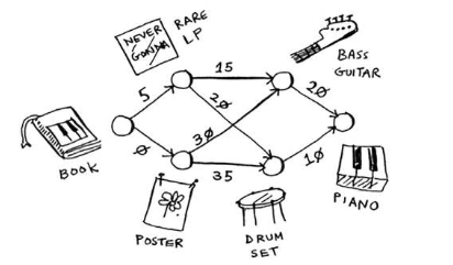
Djikstra simply works by

Look at all the nodes that we have so far and choose the node with the shortest travel distance.
Set the node as visited ( so we don’t consider it again ) - we have now found the shortest travel distance to this node
Loop through all the node’s neighbours and see if we have now found a shorter path to a new node using this new explored node.
Repeat until all nodes have been explored

We can implement djikstra using a heap as seen below

import heapq
 
def dijkstra(graph, start):
    distances = {}
    priority_queue = [(0, start)]
 
    while priority_queue:
        current_distance, current_node = heapq.heappop(priority_queue)
      
        if current_node in distances:
          continue
        distances[current_node] = current_distance
        for neighbor, weight in graph[current_node].items():
            distance = current_distance + weight
            # Unprocessed Node
            if neighbor not in distances:
                heapq.heappush(priority_queue, (distance, neighbor))
 
    return distances
 
 
test_graph = {
    'A': {'B': 1, 'C': 4},
    'B': {'A': 1, 'C': 2, 'D': 5},
    'C': {'A': 4, 'B': 2, 'D': 1},
    'D': {'B': 5, 'C': 1}
}
 
test_cases = [
    ('A', {'A': 0, 'B': 1, 'C': 3, 'D': 4}),
    ('B', {'A': 1, 'B': 0, 'C': 2, 'D': 3}),
    ('C', {'A': 3, 'B': 2, 'C': 0, 'D': 1}),
    ('D', {'A': 4, 'B': 3, 'C': 1, 'D': 0})
]
 
for start_node, expected_distances in test_cases:
    result = dijkstra(test_graph, start_node)
    assert result == expected_distances, f"Expected {expected_distances}, but got {result}"

Greedy Algorithms

Greedy algorithms are algorithms we can use to approximate a globally optimal solution. In short, we pick the locally optimal solution and in the end we’re left with the globally optimal solution.

Sometimes, greedy algorithms aren’t able to find the globally optimal solution but they allow us to get close enough. Often times, greedy algorithms will find a solution in $O (n^{2})$ time while a complete solution will take around $O (n!)$ time.

These are a class of problems known as NP-Complete.

Dynamic Programming

When thinking about dynamic programming, the goal is to identify the subproblem. Each cell in the dp table that we create is going to correspond to some subproblem of the larger problem we are trying to solve.

Knapsack Problem

Knapsack problems are when we have a bunch of choices that have an associated cost $x$ and we want to optimise for a specific quantity $Y$ .

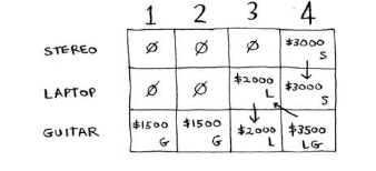
We will have to modify this approach if we wanted to get the maximum amounts for each individual item.

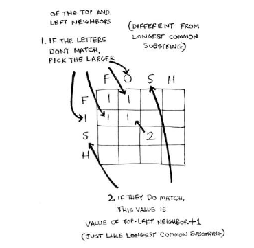
Longest Common Substring

If we have two strings eg.Hish and Fish, the longest common substring is going to be ish. How can we then compute the longest common substring?

Well, if we think about it, the answer is really

max(HIS,FIS) + 1

since hish and fish both end with a h.

If we’re trying to find the longest string between two strings that don’t share the same last character, eg. power and twerk, then the problem really is

max(power,twer) vs max(powe,twerk)

Longest Common Subsequence

How about if we want to get the longest common substring - eg. ace and abcde have the longest common substring of ace.

if the last character e matches, then it really is the question of what is the longest common substring of ac and abcd. This can then be decomposed into

max(a,abcd) vs max(ac,abc)

Since the last char matches, then we want to

Ivan's notes (Powered by 🪴 Quartz 4.0)

Table of Contents

Grokking Algorithms

Algorithms

Binary Search

Selection Sort

Memory

Arrays vs Linked Lists

Recursion

Quicksort

Merge Sort

Hash Functions

Graphs

Representations

Breadth First Search

Dijkstra’s Algorithm

Greedy Algorithms

Dynamic Programming

Knapsack Problem

Longest Common Substring

Longest Common Subsequence

Graph View

Backlinks

Ivan's notes (Powered by 🪴 Quartz 4.0)

Table of Contents

Grokking Algorithms

Algorithms §

Binary Search §

Selection Sort §

Memory §

Arrays vs Linked Lists §

Recursion §

Quicksort §

Merge Sort §

Hash Functions §

Graphs §

Representations §

Breadth First Search §

Dijkstra’s Algorithm §

Greedy Algorithms §

Dynamic Programming §

Knapsack Problem §

Longest Common Substring §

Longest Common Subsequence §

Graph View

Backlinks

Algorithms

Binary Search

Selection Sort

Memory

Arrays vs Linked Lists

Recursion

Quicksort

Merge Sort

Hash Functions

Graphs

Representations

Breadth First Search

Dijkstra’s Algorithm

Greedy Algorithms

Dynamic Programming

Knapsack Problem

Longest Common Substring

Longest Common Subsequence