Neural Networks From Scratch

Introduction §

Neural Networks §

Neural Networks are a deep learning architecture. A group of neurons are called a single layer. When we have 2 or more linear layers of neurons, we have a deep neural network.

We have a few different kinds of tasks that we might want to use neural networks for

1. Supervised Learning : When we have pre-existing labels and data points which we want our model to learn how to fit the feature space to the classification label.

2. Unsupervised Learning: When we have no explicit labels and the model finds structure in the data without the explicit labels

Back propagation arrived in 1960s but neural networks were developed in the 1940s.

Weights and Biases §

Neurons in a neural network have weights and biases. These can be thought of as knobs to tune to fit our model to the desired task. Typically, a neural network can have up to billions of adjustable parameters.

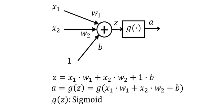
When we look at these weights and biases, they affect the neuron prediction in different ways. We can visualise this using the analogy of a graph $y=mx+c$.

Weights are like the gradient and they affect the sensitivity of the neuron to changes in the input whereas a bias can prod the network in certain directions to better fit an activation function.

Concerns §

Typically when we’re training a neural network, we’re worried about overfitting. That’s why we utilise two features

1. Batch Size : By forcing our network to update its weights w.r.t a randomly selected collection of samples, it won’t overfit to a single value.
2. Train, Test and Validate: By holding out certain portions of the data, we can make sure that our large neural network does not start memorising the data but instead begins to discover and learn certain overall patterns that are useful to make predictions.

Layer §

We typically make predictions using a layer of neurons.

These are simply a collection of neurons and form a layer. In this case, we’re using a dense layer, where every neuron in the existing layer is connected to every neuron in the preceding layer.

We can see a sample implementation as

class Layer_Dense:
  
  def __init__(self,n_inputs,n_neurons):
    # Initialize weights and biases
    self.weights = np.random.randn(n_inputs,n_neurons) * 0.01
    self.biases = np.zeros((1,n_neurons))
  
  def forward(self,inputs):
    # Calculate output values from inputs, weights and biases
    return inputs@(self.weights) + self.biases

Note here that we initialise it as (n_inputs,n_neurons) instead of (n_neurons,n_inputs) because of the ease of using self.weights in the forward pass.

When we initialise our model’s weights, typically we do two main things

• Initialise our weights randomly and close to 0 : This is to break the symmetry of weights and to ensure each weight receives different updates, and consequently will learn different features.

• Initialise our bias to 0 : This is a common approach

Terminology §

When we talk about neural networks, here are a few different bits of terminology that we need to understand

1. Array : This is a homogenous list - which is this context simply a list where every sublist has the same number and arrangement of elements.
2. List : This is just a collection of objects
3. Shape : How the array is structured
4. Tensor: An object which can be represented as an array
5. Vector : A 1 dimensional array

Linear Algebra §

There are a few different operations that we need to do in neural network training.

Dot Product §

When we look at the dot product, we need to make sure the dimensions agree. In this case, the length of r1 must be equal to the height of c1. This is simply because of the nature of the calculation.

More concretely, when performing the dot product of two matrices, the dimensions that must agree are the number of columns in the first matrix and the number of rows in the second matrix. Specifically, if the first matrix has dimensions m × n, and the second matrix has dimensions n × p, then the dot product (matrix multiplication) is defined, and the resulting product matrix will have dimensions m × p

Dot products are useful in batch inference since we can parallelise the inference step for multiple samples in a single operation.

Neural Network basics §

Activation Functions §

We use activation functions in order to allow our neural networks to map to non-linear outputs. This is because, if we had no activation functions, we would essentially have a giant linear output.

There are a few common activation functions to know

Step Function §

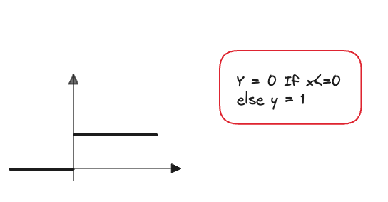A step function introduces a simple non-linearity and decides if a neuron if firing or not. However, it’s a bit too non-granular for our uses since we can’t really adjust the degree of firing

Sigmoid §

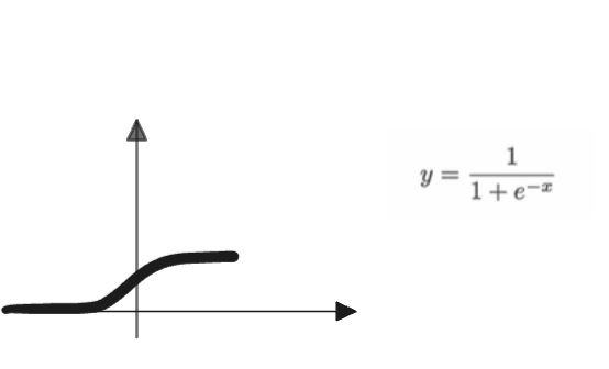
This is slightly better since we have a gradual increase in the firing rate of the neuron. Note that in this context, all values still lie between 0 and 1.

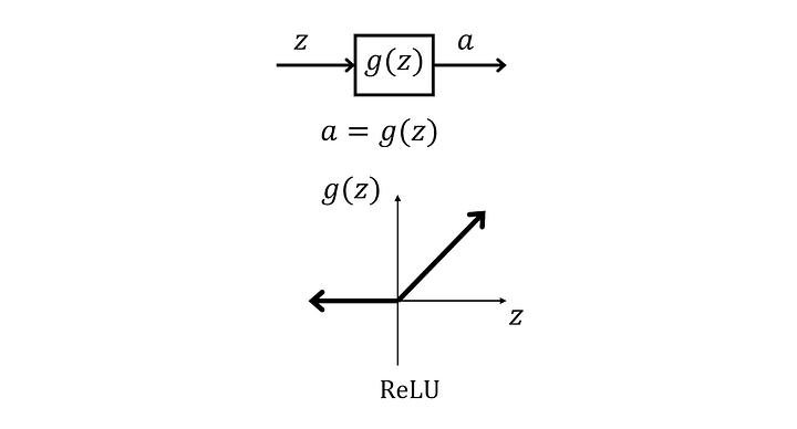
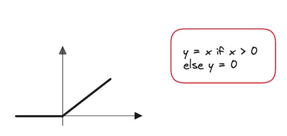
ReLU §

ReLU is very simple to compute, hence why it ended up replacing the sigmoid function in the future

Softmax §

Softmax activation function is commonly used to normalise probabilities.

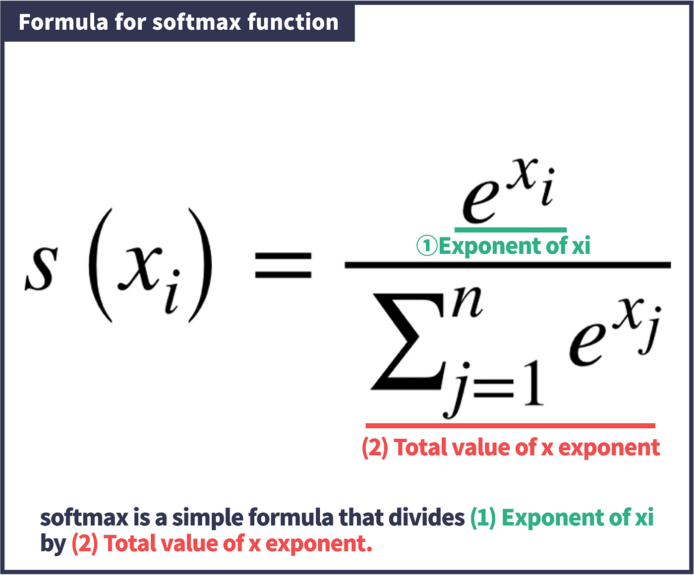
We can see an implementation below in numpy

class Activation_Softmax:
  def forward(self,inputs):
    exp_values = np.exp(inputs - np.max(inputs,axis=1,keepdims=True)) # Numerical Stability
 
    probs = exp_values / np.sum(exp_values,axis=1,keepdims=True)
 
    self.output = probs
    return probs

Since exp is a monotonically increasing function, we can prevent numerical instability by taking the max of the values and subtracting it from each value. The final value of the softmax will be the same and we avoid potential integer overflows.

Loss §

The loss function is an algorithm which determines how well the model’s predictions are working. Ideally we want it to be 0, and the more errors the model makes, the higher it should be.

Categorical Loss §

We can utilise the categorical cross entropy loss when we are dealing with multi-class classification problems.

$$L_i=-\sum _{i=0}^j{y}_{i}log({\hat{y}}_i)$$

Where $L_i$ denotes the sample loss value, $i$ the $i$-th sample in a set of $j$ possible classes, $y$ the target prediction value and $\hat{y}$ the predicted value.

Note that when we have a single class, this simply becomes the negative log likelihood.

$$L_i=-log(\widehat{y_i})$$

Since all other probabilities are going to be multiplied by 0. Normally, we clip the values by a small amount (Eg. 1e-7, 1-1e-7) so that we don’t run into integer overflow since log(0) is going to be infinity.

class Loss_CategoricalCrossentropy(Loss):
  def forward(self,y_pred,y_true):
    samples = len(y_pred)
    y_pred_clipped = np.clip(y_pred,1e-7,1-1e-7)
    if len(y_true.shape) == 1:
      correct_confidence = y_pred_clipped[range(samples),y_true]
    else:
      correct_confidence = np.sum(
          y_pred_clipped*y_true,
          axis=1
      )
    
    negative_log_likelihood = -np.log(correct_confidence)
    return negative_log_likelihood