Stanford Introduction To Statistics

Introduction §

Statistical literacy is important in data science. It establishes a rigorous framework for looking at uncertainty.

Descriptive Statistics §

It is best to use a graphical summary to communicate information since people prefer to look at pictures than at numbers.

1. Frequency/Percentage Breakdown : In such a case, it’s good to use a pie chart, bar graph or histogram so that we can see the percentage/proportion of a specific category or the relative frequency relative to other categories.
   • Histogram : We can get data on information such as density ( How many subjects fall into specific categories/specific units ) and percentages ( using the relative area )
2. Between Populations : A good choice here is a box plot ( if you have population specific data in the form of median, quartiles etc ) or a Scatterplot ( if you have pairwise data )

Numerical Summaries §

There are a few different values which we want to use to breakdown population data

1. Mean : The average when we sum up the values
2. Median : The median is the number that is larger than half of the data and smaller than the other half
3. Percentiles : The percentage of data points within the population that are lower than this data point
4. Interquartile Range : The difference between the 75th percentile and the 50th percentile
5. Standard Deviation : The average squared difference between the values in the population and the population mean

Some points to note here

If values in a population increase by a fixed amount, then standard deviation, interquartile range don’t change. Only the mean and the median increase. But, if values in a population increase by a percentage ( Eg. they all increase by 5% ), then everything will increase - s.d, interquartile range, mean and median.

Sampling §

Statistical Inference §

Some important definitions

1. Population : The entire group of subjects about which we want information from
2. Parameter : What we are trying to measure
3. Sample : The part of the population from which we collect information
4. Statistic : The estimated parameter value that we obtain from our sample

The key point here is that even a statistic from a relatively small sample will produce an estimate that is close to the actual value.

Methods §

There are a few different methods that we can use in this situation

1. Sample Of Convenience : We obtain a sample based on the most convenient ones that we can find. It tends to introduce a form of bias down the line
2. Simple Random Sample : We select subjects at random without replacement - therefore everyone has a fair chance of being selected.
3. Stratified Random Sampling : Population is divided into groups of similar subjects called strata. Then one chooses a simple random sample in each stratum.

Bias and Errors §

There are a few biases and errors that we want to avoid

1. Selection Bias : A sample that favours a certain outcome
2. Non-Response Bias : Certain populations are less likely to be represented due to their lifestyle/choices
3. Voluntary Response Bias : Certain populations are more likely to give responses (Eg. customers with bad experiences )

Therefore a good way to think about it is that

$$\text{estimate = parameter + bias + chance error}$$

Ideally, we can reduce our chance error as the sample size gets bigger.

Randomised Controlled Experiments §

We can only assign causation links using a randomised controlled experiment. This involves first setting up a treatment group and a control group.

We then do three things to limit the differences between the groups

• Double Blind : We make sure that neither the subjects nor the evaluators know the assignments to treatment and control
• Placebo: We give a placebo to the control group so that both the treatment and the control are equally affected by the placebo effect since the idea of being treated might have an effect by itself
• Randomized Assignment : This makes the treatment group as similar to the control group. Therefore we reduce the impact of individual characteristics.

Sampling Math §

When looking at sampling, there are a few different formulas we can use

We can estimate these population parameters by

Note that the standard error ( SE ) is dependent only on the size of the sample and not the size of the population.

Binomial Distribution

$E(S_n)=np$ $E(S_n)=np(1-p)$

where $n$ is the number of draws, $p$ the probability of success and $(1-p)$ the probability of failure

Calculating the Sum of n samples

$E(S_n)=n\mu$
$SE(S_n)=\sqrt{n}\sigma$

Calculating the Average

$E(\overline{X_n})=\mu$
$SE(\overline{X_n})=\frac{\sigma }{\sqrt{n}}$

Law Of Large Numbers §

Law Of large Numbers: sample mean will likely to be close to its expected value if the sample size is large. Note that this only applies to averages and percentages. It doesn’t apply to sums since the sample error increases over time.

Central Limit Theorem: It also indicates that the sampling distribution of the statistic is normal over time as the sample distribution increases no matter what the population histogram is. It only applies to draws, not a population statistic.

Requires

• We sample with replacement/we simulate independent random variables
• statistic of interest is a sum
• Min sample size is 40

Probability §

We can consider a few definitions of probability

1. Counting : The proportion of times this event occurs in many repetitions
2. Bayesian : A Subjective probability that we assign based on our own reasoning

Note that

1. Probabilities are always between 0 and 1
2. The complement of an event Eg. $P(A^{\prime })=1-P(A)$
3. Equally likely events have the same prob so just take the mean

Rules §

Addition Rule

This deals with mutually exclusive events

$$P(A\text{ and }B)=P(A)+P(B)$$

assuming that A and B are mutually exclusive

Multiplication Rule

If A and B are independent, then

$$P(A\text{ and }B)=P(A)P(B)$$

Conditional Probability §

Conditional probabilities allows us to express the probability of an event happening w.r.t the probability of a specific event

$$P(A|B)=\frac{P(A\cap B)}{P(B)}$$

This also implies that

$$P(A\cap B)=P(B)\times P(A|B)$$

The multiplication rule is simply an application of this rule since $P(A|B)=P(A)$ if two events are independent

Bayes Rule §

We have $P(A|B)$ but we want $P(B|A)$. We can calculate it by taking

$$P(B|A)=\frac{P(A\cap B)}{P(A)}=\frac{P(A|B)P(B)}{P(A)}$$

Distributions §

There are a few common distributions in most datasets

Normal Distribution §

This is a bell shaped histogram with some standard behaviour

• 68%, 95% and 99.7% of the data will fall within 1,2 and 3 standard deviations of the mean respectively.

If we have a standard normal curve, it is defined entirely by the mean and the standard deviation. We can do so by standardising the data to become a z-score.

We can approximate areas under the curve

Binomial Distributions §

We have a binary outcome from a population which we sample from. We can do so by using a binomial formula to measure the probability of $k$ successes with $n$ experiments

$$P(k)=\frac{n!}{k!(n-k)!}{p}^k(1-p{)}^{n-k}$$

We can artificially cast something to be binomial (Eg. if we have 3 outcomes then we model success as outcome A and failure as everything else )

Interestingly, as the number of experiments increases, the probability histogram of the binomial approximates the normal curve.

Random Variables §

When we’re measuring a specific quantity that is random, we call it a random variable since the value is not fixed. Instead, we can visualise its probabilities with a probability distribution. This histogram is representative of a theoretical distribution.

There are three possible histograms that you will see

1. Theoretical Distribution : The probabilities that you expect from a single event
2. Empirical Distribution : The observed outcomes
3. Sampling Distribution: The probabilities of the statistic that you expect from a single sample

Prediction §

Regression helps us to make a prediction for an independent variable given a dependent variable.

Correlation Coefficient §

The correlation coefficient shows two main things

• The direction of the correlation
• The strength of the correlation

R is always going to be -1 and 1. The sign of r gives the direction of the association and the absolute value gives the strength. Note that R only measures linear associations.

Regression §

If a scatterplot shows a linear association, then we can represent it with a line of type

$$y=a+bx$$

where $y$ is the value we’d like to predict, $x$ the value that we have and $a,b$ some values that we have to minimise. Normally we try to find a $a$ and $b$ that minimises the differences between $y_i$ ( the actual value ) and $\widehat{y_i}$ ( our predicted value ).

Regression to the mean §

Regression to the mean is a statistical phenomenon that occurs when an extreme outcome is likely to revert back to the average in subsequent measurements.

This might occur when a top scorer for instance, gets a slightly lower score in a subsequent examination. This is ultimately a normal phenomena since it is difficult to keep that edge.

Predicting §

Whenever we want to do a prediction, always put the predictor on the x-axis and proceed as on the previous slide.

Predicting y from x §

If we know $\bar{x},\bar{y},s_x,s_y,r$ then we can in turn find the regression line of $y=a+bx$ and make a prediction

Eg. If $x=41$, then what is $y$ prediction

• $\bar{x}=49.5$
• $\bar{y}=69.1$
• $s_x=10.2$
• $s_y=11.8$
• $r=0.67$

If we don’t know a value for $x$, then $y$’s best prediction is going to be the mean. If not, then we should

1. Calculate the s.d of the value below the average

$$\frac{41-49.5}{10.2}=-0.83$$

2. Next, multiply it by the $r$ value to get the new value w.r.t the mean in terms of s.d

$$-0.83\times 0.67=-0.5561$$

3. Calculate the new value

$$69.1-0.5561\ast 11.8\approx 62.5$$

Predicting X from Y §

Eg. If $y=79$, then what is $x$ prediction

• $\bar{x}=49.5$
• $\bar{y}=69.1$
• $s_x=10.2$
• $s_y=11.8$
• $r=0.67$

Calculate the s.d of the value below the average

$$\frac{79-69.1}{11.8}\approx .84$$

2. Next, multiply it by the $r$ value to get the new value w.r.t the mean in terms of s.d

$$0.84\times 0.67=0.5628$$

3. Calculate the new value

$$49.5+0.5628\ast 10.2\approx 55.2$$

Normal Approximation §

Normal approximation in regression refers to the assumption that the distribution of errors or residuals in a regression model follows a normal distribution

We can use it to determine given a $x$ value, what is the percentage of students that obtained scores between a range of $y_a$ to $y_b$.

From regression, we know the average (the predicted value for a specific x), and the normal approximation tells us more about the actual values for a specific x and how they look like, as they follow a normal curve.

Residuals §

The differences between observed and predicted y-values are called residuals. We can use residuals to determine whether the use of regression is appropriate. If a curved pattern is observed ( when residuals plotted against independent variable ), then it indicates that regression might not be the best option.

If the residuals follow a fan shape, then it’s also a problem since it indicates an increasing variance over time.

When we see large outliers in our dataset with huge residual values, they might in turn represent typos or interesting phenomena. A point away from the mean has high leverage - it can cause a big change on the regression line.

Confidence §

Note that just because something is statistically significant, does not mean the the effect size is important. A large sample size $n$ makes any small increase or decrease from the mean statistically significant.

A 95% confidence interval contains all values for the null hypothesis that will not be a two-sided test at a 5% significance level

We have two possible kinds of errors

• Type 1: When we incorrectly reject our null hypothesis
• Type 2: When we incorrectly accept our null hypothesis

Confidence Intervals §

Confidence intervals are a way for us to express our computed sample percentage in terms of the standard error.

Eg, we have a prediction of 58% and we know the SE is 1.6. Therefore, we can express it in terms of a standard error range with a 95% confidence interval as

$$[54.8,61.2]$$

Note that the interval varies from sample to sample while the population percentage is a fixed number.

Bootstrap §

We can use a bootstrap approach in order to estimate the population standard deviation. The formula to use is

$$\sigma =\sqrt{p(1-p)}$$

which we can then use to calculate a SE of a given sample size using

$$SE(S)=\frac{\sigma }{\sqrt{n}}$$

To decrease the confidence interval width, we could either increase sample size or decrease confidence level.

Hypothesis Tests §

We use a hypothesis test to determine if there is sufficient evidence to reject the null hypothesis. Note that our goal in most cases is to find enough evidence that the null hypothesis can be rejected.

We always start with 2 hypothesis

• Null Hypothesis : All is fine
• Alternative Process : There is a different chance process which is generating the data

Eg. We toss a coin 10 times and get 7 tails. Is the coin biased?

$H_0$ : Indicates that the $P(T)$ is indeed $\frac{1}{2}$. $H_A$: Indicates that $P(T)\ne \frac{1}{2}$

We can have either one-sided hypothesis tests or two-sided hypothesis tests.

If we want to extend our hypothesis test to be able to accomodate two-samples ( from two separate events ), the standard error for two independent events is simply their squared sum.

Test Statistic §

We use a test statistic to determine how likely it is to get the observed statistic if $H_0$ was true. We do so using the $z$ statistic, which is simply

$$\frac{\text{observed - expected}}{SE}$$

Larger values of $z$ indicate a stronger piece of evidence. We calculate a $p$ value using normal approximation, which tells us the probability of getting the value.

We normally use a 5% significance value to determine this. Note that the p-value does not determine the probability that $H_0$ is true. This is because $H_0$ is either true or not.

T-Test §

When we don’t know $\sigma$ or when the sample size is small ($n<20$ ), we need to use the $t$ - distribution with $n-1$ degrees of freedom for our $n$ samples.

In this case, we use our $t$-distribution to estimate

• The confidence interval ( since we don’t have a $z$-score that we can use to determine the range ) using a $t_{n-1}$ score
• The standard deviation of the curve

Matched Pairs §

Sometimes, we might not be able to use a $t$-test or a $z$-test when we have two populations that are not independent from each other. (Eg. Husband and wives ages).

In this case, we can analyze the difference between each pair with a regular t-test.

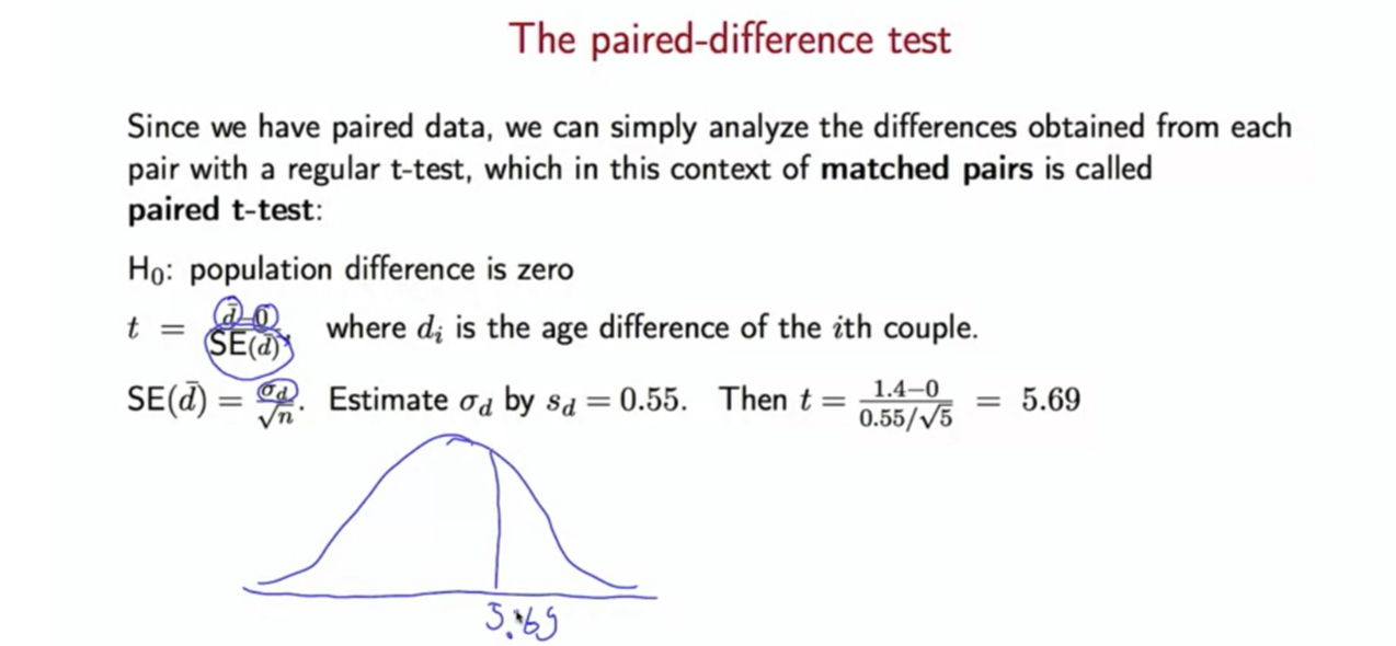
The independence here is the sampling of the couples, not their ages.

Simulations §

We can use simulations in order when we want to get some statistic $\theta$ which cannot be approximated using the normal distribution.

Monte Carlo §

The law of large numbers means that when we have a large sample size, we can accurately approximate a population statistic.

$$SE(\hat{\theta })=\sqrt{E(\theta -E(\hat{\theta }){)}^2}$$

We can use the monte carlo method by simply

1. Taking many samples of a series of draws (Eg. 1,000 samples of 100 observations )
2. Computing $\hat{\theta }$ for each sample, resulting in ${\theta }_1,{\theta }_2,\dots ,{\theta }_n$ observations
3. Compute the standard deviation of these series of draws which in turn approximates the standard error of the statistic that we have computed

$$S({\hat{\theta }}_1,\dots ,{\hat{\theta }}_n)=\sqrt{\frac{1}{n-1}\sum _{i=1}^n({\hat{\theta }}_i-avg({\hat{\theta }}_i){)}^2}$$

This method only works if we can sample a large amount of samples of size 100. This works since the sample distribution will be close to the population distribution.

Bootstraps §

There are two main kinds of bootstrapping

Non-Parametric Bootstrap §

If we cannot sample from the population, then we can use the plug-in principle and sample from the population instead. This means that we draw $n$ times with replacement from $X_1,\dots ,X_n$ which represents a collection of $n$ samples that we have from the population itself.

We might also utilise a percentile interval. The bootstrap percentile interval is more useful for skewed bootstrap histograms because it is a non-parametric method that does not rely on the assumption of a normal distribution.

Parametric Bootstrap §

Sometimes, a parametric model is more appropriate for the data - which simulates a bootstrap sample from this model with an unknown mean and standard deviation.

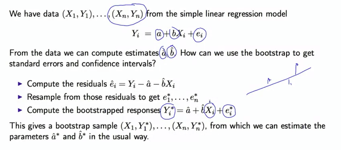
Bootstrapping Residuals §

We might instead use the residuals to compute standard errors. We can do so by computing our individual residuals, then resampling from the residuals to get a random sample of error terms.

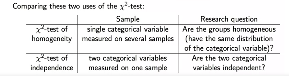
Categorical Data §

Test Type	Purpose	Variables Involved
Goodness-of-Fit	Determine if a variable comes from a specified distribution	One categorical
Independence	Check if two categorical variables are likely to be related or not	Two categorical
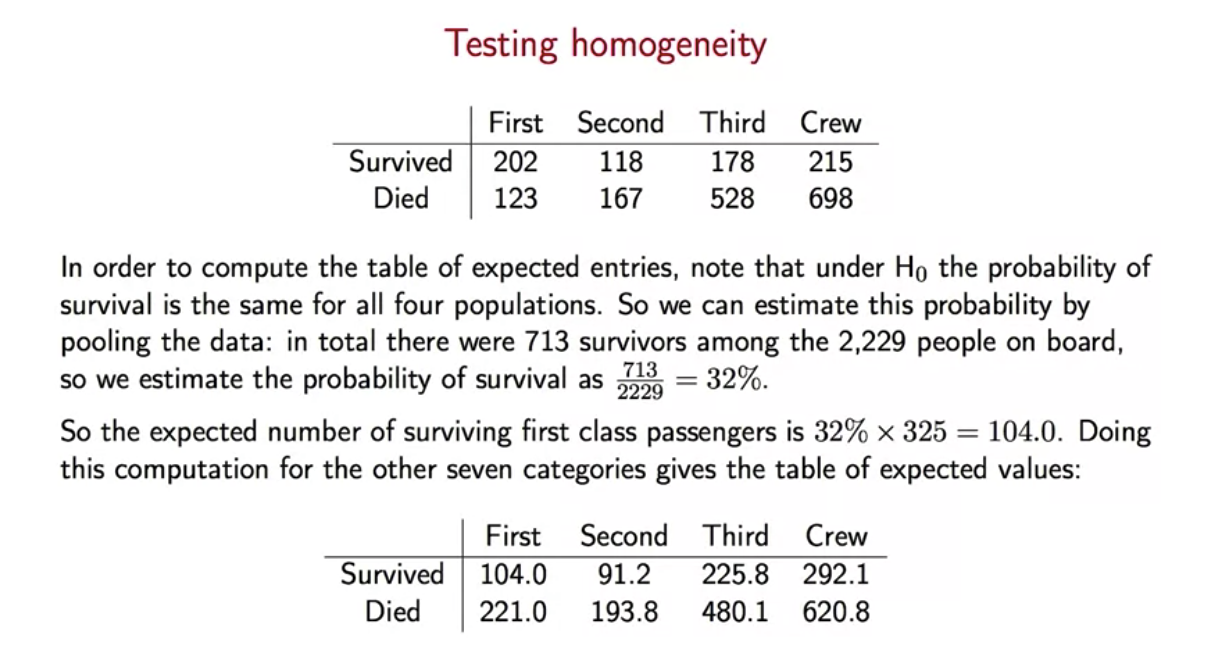
Homogeneity	Determine if frequency counts are distributed identically across different populations	One categorical

For instance, goodness-of-fit might be used to determine if a certain distribution is observed across the different categories ( according to a manufacturer’s percentage for instance ) while homogeneity might try to determine if all of the categories have equal frequency/percentage counts.

Chi-Square Statistic §

How can we make predictions for categorical variables - or even calculate whether the categorical distribution holds. We can do so using a goodness of fit test.

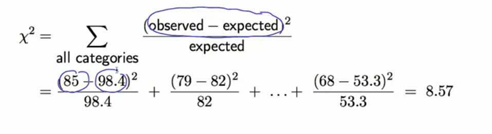This is a statistic called ${\chi }^2$. The larger the value, the greater the evidence against $H_0$. The p-value is then the right-tail of the ${\chi }^2$ distribution with degrees of freedom = number of categories - 1.

Using it for Homogeneity and Independence §

Anova §

Analysis Of Variance ( ANOVA ) is used as a parametric test to determine if there is a statistically significant difference in outcomes between 3 or more groups. ANOVA tests for a difference overall but you cannot determine which of the groups is statistically significant.

We use the F-statistic to determine the variation between the groups.

$$F=\frac{MST}{MSE}$$

If the groups are equal in terms of outcomes, then the ratio should be around 1. Otherwise, it will not be exactly 1. This statistic follows a F-distribution with $k-1$ and $N-k$ degrees of freedom.

Anova makes the following assumptions

1. Each group sample is drawn from a normally distributed population
2. Variances across the group are approximately equal
3. Data is independent
4. Dependent variable must be continuous ( Quantitative ) and independent must be categorical

It is important to check these assumptions before we proceed to do an anova analysis. Remember that Anova can only conclude that the group means are not equal.

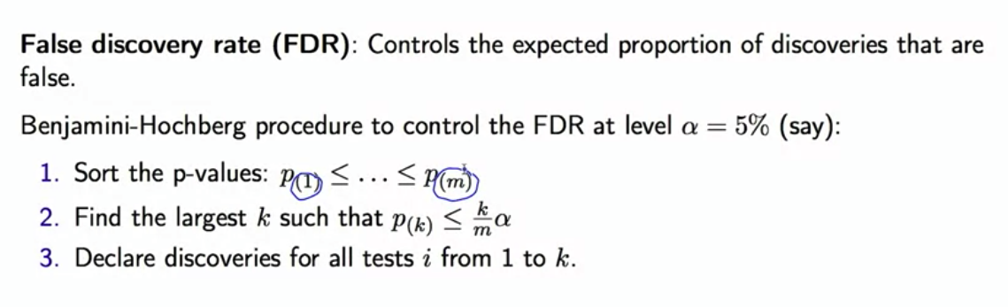
Data Snooping and Reproducibility §

A p-value of 5% indicates that there is a 5% chance to get a highly significant result if there is no effect. This means that if we do 800 tests, then even if there is no effect at all, we expect to see 800 * 0.05 = 40 significant tests just by chance.

This is known as the multiple testing fallacy and has led to a crisis with regard to replicability and reproducibility.

• Replicability : We get similar conclusions when working with different samples, procedures and data analysis methods
• Reproducibility : We get the same results when we use the same data and data analysis methods

Bonferroni correction §

If there are $m$ tests, then multiply the p-values by $m$. This is a very restrictive guard which presents you from having even one false positive among the $m$ tests

False Discovery Proportion §

This can be be calculated by using the formula of

$$\text{FDP}=\frac{\text{Number of false discoveries}}{\text{total number of discoveries}}$$

FD