Zero To Hero

Zero to Hero is a course by Andrej Karpathy which focuses on helping people to understand the math behind deep learning networks. It’s a pretty fantastic course and I highly recommend it.

Micrograd §

Introduction §

Micrograd is a simplified implementation of scalar back propagation written in numpy and python.

Notebook with code on how to implement this is here

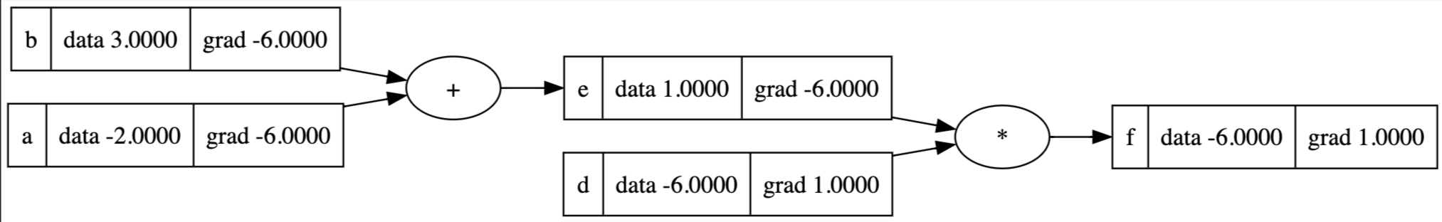
A good way to think about Back Propagation is the flow of gradients through a network of operations.

We can resolve the gradients for some equations symbolically - i.e. we can solve them by solving for an abstract form that they match and then derive the gradients.

Operations Supported §

Here is a list of some simple equations that our micrograd implementation supports

Original Equation	$\frac{da}{da}$	$\frac{db}{da}$	$\frac{dc}{da}$
a = b + c	1	1	1
a = b * c	1	c	b
a = tan(b)	1	1 - $a^2$	nil
$a=e^x$	1	e^{x}	nil
$a=\frac{b}{c}$	1	$\frac{1}{c}$	b
$a=b^n$	1	$c\times b^{c-1}$	nil ( n is treated as a constant here)

Chain Rule §

But we don’t just want a simple $a=b+c$ , we probably want to compute a more complex equation such as

a = 3
b = 3
c = a * b

d = 12
e = 3
f = 12 + 3

z = c * f

and from there calculate the value of

$$\frac{dz}{da}$$

We can’t do this using our original formula but we can do so using the chain rule, which states that

$$\frac{dz}{da}=\frac{dz}{dc}\ast \frac{dc}{da}$$

And so if we chain many of these operations together, we eventually get the gradient we want - that is the change in the loss with respect to some value that’s much further down the original chain of equations.

The important thing to note here is that we can therefore compute the derivative for every single one of these variables by recursively applying the chain rule and finding the product of it with the local derivative that you are calculating.

Applications §

Ultimately when we have a whole cluster of these values together, we can form neural nets, which can be represented as matrix multiplication (see code for implementation)

Bigram Models §

A Bigram is simply a collection of two characters (Eg. ab,de ) and a Bigram model in this course is simply a model which takes in an input of two characters and then outputs a prediction of the next most likely token.

Karpathy outlines two ways to create these Bigram models

1. Generating manual counts : We simply break our entire sample of words into two character chunks

2. Neural Networks : We initialise a network with roughly equal weights at the start and use stochastic gradient descent to slowly arrive at the same probabilities that we obtained in our manual counts process

Neural Network Approach §

Using a bigram model is intuitive because we have a list of $j$ counts that we can then convert to probabilities by

$$c_i=\frac{c_i}{{\sum }_{j=0}^n{c}_j}$$

How then can we obtain the same effect using neural networks? On a high level, we can do so using a single Neuron

Neuron §

A neuron in a neural network simply takes in a vector as input and spits out a vector as input using the formula

$$y=W\times X+b$$

Where $W$ is the weights of the network and $b$ the bias of the neuron. We can think of the weights and biases as knobs we can tune in order to get the final result we want

Neurons and Bigrams §

There’s a small problem with $y$. It’s that

1. It doesn’t sum to 1 nicely
2. It has some negative numbers from time-to-time

What we want is a vector with $j$ values that sum to 1 nicely so we can make a prediction using a multinomial prediction. Therefore, we can solve this by simply doing

$$y_i\prime =\frac{e^{y_i}}{{\sum }_{j=0}^n{e}^{y_j}}$$

So, what we want is a slightly modified form of y. So, what then can we compare $X$, $W$ and $b$ to?

• X is going to be a one-hot encoded value for the first character of the bigram (Eg. we chose a a, what are the respective probabilities for ab,aa and so on? )
• W is going to be a randomly initialised set of values that range from $-\infty \to \infty$, since our counts originally ranged from $0\to \infty$ , we can simply consider $W$ as our log counts since the log function takes positive numbers and then maps them to the same range that $W$ occupies

Loss Function §

All that’s missing now is a Loss Function. This is a function which is used to measure the quality of our model’s predictions. The better the prediction, the lower the loss should be

Ideally, if we choose the wrong character, we want the probability to be 0. If we’ve chosen the right character, we want the probability to be 1. Therefore, we want a function which can do this given the probability of the respective character we’ve predicted in $y$.

We are going to use the Negative Log Likelihood of the generated probability of the right choice as a loss function because

1. If our model knows exactly what is going to be next, it will assign a probability of 1.
2. If our model has zero information, then everything will be equally likely - so prob will be 1/27
3. Probabilities are solely from 0 to 1
4. Log(1) = 0 , log(0) = -inf therefore the range of each value will be -inf <= x <= 0
5. -log(1) = 0, -log(0) = inf, therefore as model becomes more accurate, our loss tends to 0

Batch Size §

We can now train our model! Some key concepts here to consider when training our model are

1. Batch Size: We don’t want to pass the entire dataset when we train the model, therefore we utilise a subset of the dataset when doing the forward pass and the back propagation.

2. Model Smoothing: When we train our model, we want our weights to be small to prevent overfitting. Therefore, we can modify our loss function to favour smaller weights using an additional term of $ϵ\times w.mean()$

Multi Layer Perceptron §

A Multi Layer Perceptron is a neural net with an input layer, one or more hidden layers and an output layer. In our case, we increase the context size from 2 to 3 to create a new prediction layer.

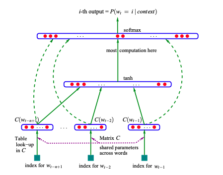
Embeddings §

Instead of mapping our characters to probabilities, we utilise embeddings. These are real number vectors used to represent semantic meaning that our model learns over the course of its training. it also means that we can be more flexible in our block size, potentially increasing the context length by utilising a larger vector of concatenated embeddings.

Hyper-parameter tuning §

We can utilise hyper parameter tuning as a way for us to explore the entire training set to find an efficient learning rate to train our model with. Remember that the learning rate is the amount that we adjust our model’s weights by.

There are three main ways that we can do so

1. Learning Rate Decay : We can decay our model’s learning rate over time so that we do not have such major updates.

2. Learning Rate Exploration : We can run small experiments whereby we iteratively increase the learning rate with each epoch. This allows us to see roughly how changes in the learning rate can affect the loss of our model.

3. Train, Test and Validation: We can also split up our dataset into a train , test and validation set. This is useful because with enough epochs, our model will start to memorize the data it has been given. Therefore, we hold out a bit of the data in the form of a validation set. If our model has roughly the same performance on the validation and training set, then it probably hasn’t overfitted on the data yet.

Building GPT §

Here is a transformer

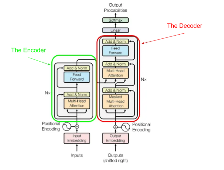
Attention §

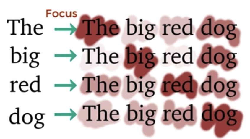
Attention is a mechanism which helps our neural network to extract more complex information from a given token sequence. In our example below, we have an example of self-attention since our model learns to weight the importance of different positions within a single input sequence when computing its representation.

There are two main forms of attention that might exist in a Transformer

• Self-Attention : Our attention network only focuses on the set of nodes that it has been given
• Cross-Attention: Our attention network focuses on the set of nodes it has been given and another source of input which is out of its network block.

Positional Vectors §

Attention is simply a set of vectors - it doesn’t have any notion of space. That’s why we utilise a positional encoding to include in this information to the vectors that Attention is working on.

Simplified Masked §

Eg. Simple Attention where we take the average of all past tokens and existing token

x = [1,2,3]
x' = [1,1.5,2]

We can derive x' from x by taking

a = [[1 0 0],[1 1 0],[1 1 1]]
a /= a.sum(a,1,keepdim=True)
or
a = F.softmax(wei,dim=-1)
a@x'.T = [1,1.5,2]

Query, Key and Vector §

A good way to think about the query and key vector is that of attention. We want to be able to obtain a matrix which tells each token how much to weight previous tokens (Eg. A vowel might want to look for a consonant)

$$1+2+3+\cdots +n=\frac{n(n+1)}{2}$$

In short

• Query : What I’m looking for
• Key : What I can offer
• Value : What I actually offer

$$softmax(\frac{Q\times K^T}{\sqrt{d_k}}+M)\times V$$

where

• $d_k$ is a normalising factor in this case so that we can ensure that our final resulting variable has unit variance and mean. If not softmax will converge to one-hot vectors.
• M is an optional mask.
• V is a value vector which is matrix multiplied against our resulting softmax value

We can see this in an implementation below where we apply an optional mask to our generated attention vector which is a $T\times T$ vector. We can choose to note apply a mask if we’re doing things like sentiment analysis or translation where we want the attention mechanism to have access to the entire set of tokens.

# let's see a single Head perform self-attention
head_size = 16
key = nn.Linear(C, head_size, bias=False)
query = nn.Linear(C, head_size, bias=False)
value = nn.Linear(C, head_size, bias=False)
k = key(x)   # (B, T, 16)
q = query(x) # (B, T, 16)
wei =  q @ k.transpose(-2, -1) # (B, T, 16) @ (B, 16, T) ---> (B, T, T)

tril = torch.tril(torch.ones(T, T))
wei = wei.masked_fill(tril == 0, float('-inf'))
wei = F.softmax(wei, dim=-1)

Multi-Head attention §

When computing the value of an attention mechanism, if we apply the same transformation across multiple heads running in parallel, then it’s a multi-head attention. Multi-head attention is therefore similar to that of a convolution layer.

We also add in a projection linear layer after we finish up the multi-head

We can see an implementation below as

class Head(nn.Module):
    """ one head of self-attention """
 
    def __init__(self, head_size):
        super().__init__()
        self.key = nn.Linear(n_embd, head_size, bias=False)
        self.query = nn.Linear(n_embd, head_size, bias=False)
        self.value = nn.Linear(n_embd, head_size, bias=False)
        self.register_buffer('tril', torch.tril(torch.ones(block_size, block_size)))
 
    def forward(self, x):
        B,T,C = x.shape
        k = self.key(x)   # (B,T,C)
        q = self.query(x) # (B,T,C)
        # compute attention scores ("affinities")
        wei = q @ k.transpose(-2,-1) * C**-0.5 # (B, T, C) @ (B, C, T) -> (B, T, T)
        wei = wei.masked_fill(self.tril[:T, :T] == 0, float('-inf')) # (B, T, T)
        wei = F.softmax(wei, dim=-1) # (B, T, T)
        wei = self.dropout(wei)
        # perform the weighted aggregation of the values
        v = self.value(x) # (B,T,C)
        out = wei @ v # (B, T, T) @ (B, T, C) -> (B, T, C)
        return out
 
class MultiHeadAttention(nn.Module):
    """ multiple heads of self-attention in parallel """
 
    def __init__(self, num_heads, head_size):
        super().__init__()
        self.heads = nn.ModuleList([Head(head_size) for _ in range(num_heads)])
 
    def forward(self, x):
        return torch.cat([h(x) for h in self.heads], dim=-1)

Note that each head will cast our original embedding dimension to head_size. Therefore in this specific implementation, we need to divide the embedding dimensionality by 4 to get the size of the head for each multi head.

Note that our head will cast our final resulting output of tokens to have an embedding dimension head_size ( using the val matrix )

We can then concatenate the resulting outputs together to get a new result. This allows the model to attend to different aspects of the input representation simultaneously, capturing different relationships between tokens in the input sequence

Feed Forward §

A feed forward layer is a simple Multi Layer Perception (MLP) which provides a simple linear layer followed by a non-linear activation function. Interestingly, we scale up the inner layer by 4 before scaling it down.

class FeedFoward(nn.Module):
    """ a simple linear layer followed by a non-linearity """
 
    def __init__(self, n_embd):
        super().__init__()
        self.net = nn.Sequential(
            nn.Linear(n_embd, 4 * n_embd),
            nn.ReLU(),
            nn.Linear(n_embd*4,  n_embd),
        )
 
    def forward(self, x):
        return self.net(x)

Layer Normalisation §

Layer Normalization is a technique used to normalize the rows. It’s slightly better than batch norm in this case because

1. We don’t need to keep a running count of the mean and variance ( since we do a calculation for each independent calculation )

2. Normalisation is easier to perform

Essentially, it’s meant to help make the outputs be unit gaussian.

Dropout §

We can utilise Dropout as a way to help prevent our network from overfitting. The overall intuition is that by disabling certain networks within our overall network during the training, we end up creating an ensemble of sub networks that are combined during inference to make better predictions